Chapter 1. Introduction

Following the release of Qucs-0.0.18 in August 2014 the Qucs Development Team considered in detail a number of possible directions that future versions of the software could take. Spice4qucs is one of these routes. It addresses a number of problems observed with the current version of Qucs while attempting to combine some of the best features of other GPL circuit simulation packages. The project also aims to add additional model development tools to those currently available in Qucs-0.0.18. Qucs was originally written as an RF and microwave engineering design tool which provided features not found in SPICE, like S parameter simulation, two and multiport small signal AC circuit analysis and RF network synthesis. Since it was first release under the General Public License (GPL) in 2003 Qucs has provided users with a relatively stable, flexible and reasonably functional circuit simulation package which is particularly suited to high frequency circuit simulation. In the years following 2003 the Qucs Development team added a number of additional simulation facilities, including for example, transient simulation, device parameter sweep capabilities and single tone Harmonic Balance simulation, making Qucs functionality comparable to SPICE at low frequencies and significantly extended at high frequencies. Considerable effort has also been made to improve the device modelling tools distributed with Qucs. The recent versions of the software include code for algebraic equation manipulation, Equation-Defined Device (EDD) modelling, Radio Frequency Equation-Defined Device (RFEDD) simulation and Verilog-A synthesised model development plus a range of compact and behavioural device modelling and post simulation data analysis tools that have become central features in an open source software package of surprising power and utility.

One of the most often requested new Qucs features is “better documentation”, especially documentation outlining the use and limitations of the simulation and the modelling features built into Qucs. Qucs is a large and complex package which is very flexible in the way that it can be used as a circuit design aid. Hence, however much documentation is written describing its functionality there are always likely be simulation and modelling examples that are missing from the Qucs documentation. In future Qucs releases will be accompanied by two or more basic Qucs documents. The first of these, simply called “Qucs-Help”, provides introductory information for beginners and indeed any other users, who require help in starting to use Qucs. The second Qucs document, called “Spice4qucs-Help”, introduces more advanced simulation and modelling topics. Both documents present a large number of typical circuit simulation and compact device modelling examples. In the text these are also linked to sets of Qucs reference material. Since 2003 the Qucs Development Team, and other authors, have published a body of work concerning Qucs and its applications. A bibliography of these publications can be found at the end of this document. Anyone interested in learning about Qucs is recommended to read these publications as they provide a wealth of information on basic and advanced Qucs topics. Both the “Qucs_Help” and “Spice4qucs-Help” documents are very much work in progress. Updated versions will be published with each new Qucs release. Moreover, to keep everyone up to date with Qucs current developments it is planned to updated them during future Qucs development phases. The latest documentation can be found at https://github.com/Qucs/qucs-help.

1.1 Background

The current rate of Qucs downloads from http://qucs.sourceforge.net/ is around 3000 per week with a total of roughly 1.5 million downloads since Qucs was first released in 2003. This figure does not however, imply that 1.5 million copies of Qucs are currently in regular use. It does perhaps give an indication of the popularity of the software, particularly amongst users interested in RF circuit design and simulation. For a high percentage of regular Qucs users the current distribution version (Qucs 0.0.18) provides a reasonably stable and accurate simulation tool equipped with more than enough facilities to meet their everyday needs. In reality Qucs is not perfect but includes a number of weaknesses and known limitations. The onward march of technology also makes it imperative that Qucs evolves from a traditional circuit simulator to a design tool that can handle modelling and simulation of circuits which include devices from new emerging technologies. Today Qucs includes an extensive range of component, device and circuit modelling tools, allowing it to model and simulate circuits built from standard components and new production devices.

Three of the primary aims of the work undertaken by the Qucs Development Team are firstly to remove software bugs and improve the overall performance of the package, secondly to address known weaknesses and limitations and thirdly to develop the package by adding features which increase it’s utility. Readers who are not familiar with open source software development may be unaware of how the development process works. By “Qucs Development Team” we mean a group of interested individuals who freely give both their time and expertise for the improvement of the GPL Qucs package. The Qucs Development Team is not a fixed group but is a dynamic organisation where different people contribute, simultaneously or at different times, to the same part or different parts of the software. The spice4qucs project group is one of a number of sub-groups within the overall Qucs Development Team. It was formed to address the known limitations of the previous Qucs releases and to take advantage of the work done by other GPL circuit simulation teams working on the Ngspice ( http://ngspice.sourceforge.net/ ), Xyce ( https://xyce.sandia.gov/ ) and SPICE OPUS (http://www.spiceopus.si/) circuit simulators.

The spice4qucs initiative is an ongoing project which attempts to:

1. Correct known weaknesses observed with the current Qucs analogue simulation engine “qucsator”. Qucsator is based on classical numerical mathematics routines for the solution of electrical network linear and non-linear real and complex algebraic equations and time domain algebraic and differential equations. For small circuits, qucsator works well in the DC and AC small signal domains. However, in the transient and Harmonic Balance simulation domains it can fail to converge to an acceptable solution. Its performance is also often below that expected of a modern circuit simulator employing sparse matrix algorithms. However, qucsator works well for RF small signal AC simulation and will for some time remain the first choice for this simulation domain.
2. Provide Qucs users with a choice of simulation engine selected from qucsator, Ngspice, Xyce and SPICE OPUS. By selecting Ngspice, Xyce or SPICE OPUS as the Qucs simulation engine users may capitalise on all the features offered by the extensive SPICE developments which have taken place over the last forty years. Both Ngspice, Xyce and SPICE OPUS offer improved transient simulation convergence and speed, particularly for large non-linear circuits. Xyce brings an alternative implementation of single tone Harmonic Balance simulation to Qucs which offers much improved convergence properties for both linear and non linear components and devices. The latest version of Xyce, 6.5 at the time of writing, also offers multi-tone Harmonic Balance simulation. SPICE OPUS adds transient shooting methods for the steady state analysis of large signal AC simulation and optimization.
3. Extend Qucs subcircuit, Equation-Defined Device (EDD), Radio Frequency Equation-Defined Device (RFEDD) and Verilog-A device modelling capabilities. The latest spice4qucs release (Qucs-0.0.19-S) offers much improved component and device modelling features that work as interlinked tools, supporting model development as a continuous flow from physical concept to compiled C/C++ code. This feature is centred around a “turn-key” version of the XSPICE Code Model construction tools. If required the spice4qucs project can also use the Berkeley “Model and Algorithm Prototyping Platform” (MAPP http://draco.eecs.berkeley.edu/ dracotiki/tiki-index.php?page=MAPP ) for compact model construction. It is also possible to synthesis Ngspice, Xyce SPICE OPUS SPICE netlists from Qucs EDD and RFEDD models and to synthesise Verilog-A models from Qucs EDD and SPICE B components.
4. Offer Qucs users access to the additional simulation tools and extra component and device models provided by Ngspice, Xyce and SPICE OPUS. This includes much improved component library facilities which allow the use of device manufacturers SPICE models and XSPICE Code Models.
5. Offer for the first time with Qucs a true mixed-mode analogue-digital circuit simulation capability using Qucs/Ngspice/SPICE OPUS/XSPICE simulation.

The spice4qucs initiative is an on going project and must be considered as very much work in progress. In its early releases not all the features listed above will be available for public use. It is however, the intention of the Qucs Development Team to introduce them as quickly as possible. Other features not listed in the previous entries may also be introduced.

1.2 Qucs-0.0.18 Structure

A block diagram showing the main analogue modelling and simulation functions of the Qucs-0.0.18 package is illustrated in Figure 1.1. For convenience, particularly easy identification, blocks with similar modelling or similar simulation functions have been coded with identical colours, for example dark red indicates the GUI and qucsator analogue simulation engine and dark green major component and device modelling tools. The direction of the flow of data between blocks are also shown with directed arrows. Central to the operation of the Qucs-0.0.18 package is the Qucs graphical user interface (GUI), the qucsator simulation engine and a post simulation data processing feature (indicated by the yellow block in Figure 1.1) for the extraction of device and circuit parameters and the visualisation of simulated signal waveforms. Cyan blocks in Figure 1.1 identify the well known Octave numerical analysis package ( https://www.gnu.org/software/octave/ ). Qucs employs Octave for additional post simulation data processing and waveform visualisation plus an experimental circuit simulation process where qucsator and Octave undertake cooperative transient circuit simulation (cyan coloured blocks). The single light brown block in Figure 1.1 represents the ASCO optimisation package which is used by Qucs for determining circuit component values and device parameters which result in specific circuit performance criteria.

Readers who are not familiar with the basic operation and use of the Qucs GUI, circuit simulator and output processing routines should consult the “Qucs-Help” document before proceeding further with this more advanced document.

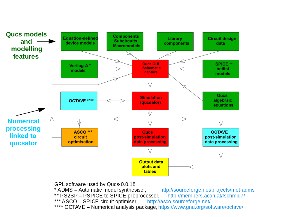
Figure 1.1. A block diagram showing the analogue modelling and simulation facilities provided by Qucs-0.0.18.

1.3 Qucs future capabilities

Figure 1.2. presents an extended version of the Qucs-0.0.18 functional diagram where the added blocks indicate areas chosen for current and future Qucs development. Two major extension to Qucs functionality are obvious, namely the addition of the Ngspice, Xyce and SPICE OPUS circuit simulators to the Qucs package and the increase in the Qucs device modelling capabilities through the addition of the XSPICE Code Modelling software. Figure 1.2. only gives a rough picture of the proposed changes to Qucs under development by the spice4qucs project. Much of the detail will become clearer later in the manual text and reference sections.

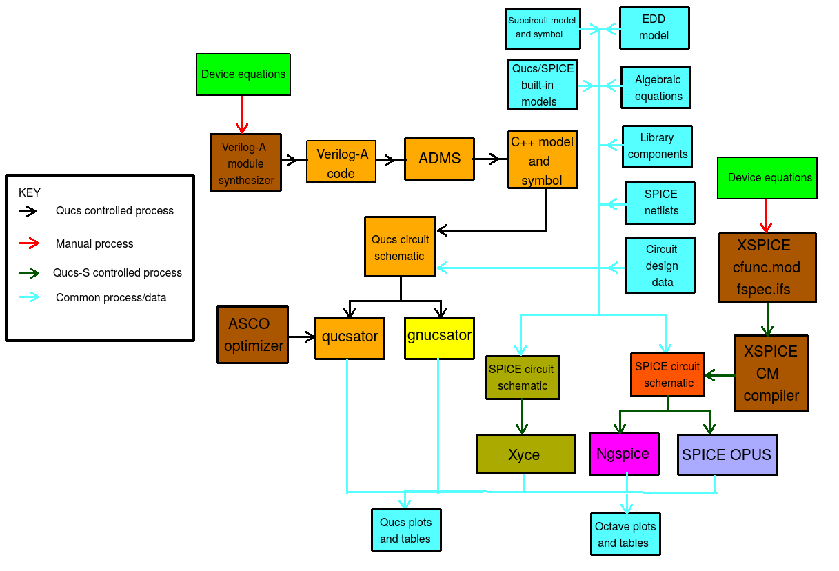
Figure 1.2. An block diagram outlining the extended Qucs-S simulation and modelling tools under development by the spice4qucs initiative.

1.4 A first view of the extended spice4qucs device modelling and simulation features

At this point it seems appropriate to introduce a short example which demonstrates how much Qucs has evolved since the release of version 0.0.18. This example has been deliberately chosen to present an overview of the major new Qucs features either already developed by the spice4qucs project or planned for future releases. To provide readers with adequate information on how to make the best use of the new spice4qucs features they are described in detail in later chapters of this document.

Qucs version 0.0.18 is a surprisingly sophisticated program with quite a number of hidden features which are not obvious to most Qucs users. Given in Figure 1.3 is a Qucs schematic which demonstrates a little known application of the circuit simulator. Qucs is ideal for developing high level behavioural models of new components or devices which are not implemented in the distributed software. The schematic in Figure 1.3. introduces the physical equations and device parameters for a semiconductor tunnel diode. By using the Qucs parameter sweep and DC simulation operations it is possible to scan the diode bias voltage Vpn, calculate the tunnel diode bias current Ipn at each bias point and plot the device id = f(vd) characteristics. Note that in this introductory example the Qucs schematic does not include any electrical components. Moreover, the tunnel diode current is calculated directly from its physical model_equations and model_parameters.

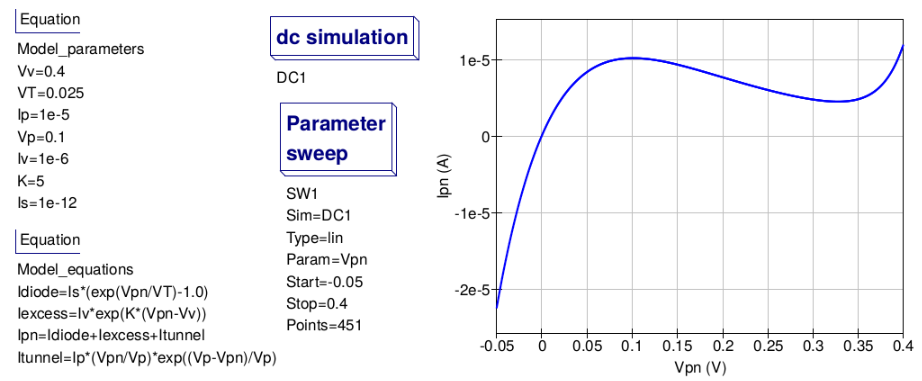
Figure 1.3. Mathematical representation of Id = f(Vd) for a semiconductor tunnel diode, including device model_parameters, model_equations and a Qucs DC scan test.

The Berkeley Model and Algorithm Prototyping Platform (MAPP) is a new GPL modelling and simulation tool. It is developed by the MAPP team at the Department of Elecrical Engineering and Computer Science, University of California, Berkeley using a MATLAB (copyright) subset common to the Octave numerical analysis software. As part of the spice4qucs project the MAPP software has been interfaced with the Qucs GUI. Figure 1.4 introduces a MAPP behavioural model for the tunnel diode in Figure 1.3. Notice how similar the models in Figures 1.3 and 1.4 are. MAPP circuit simulation results in the diode characteristic plotted in Figure 1.4.

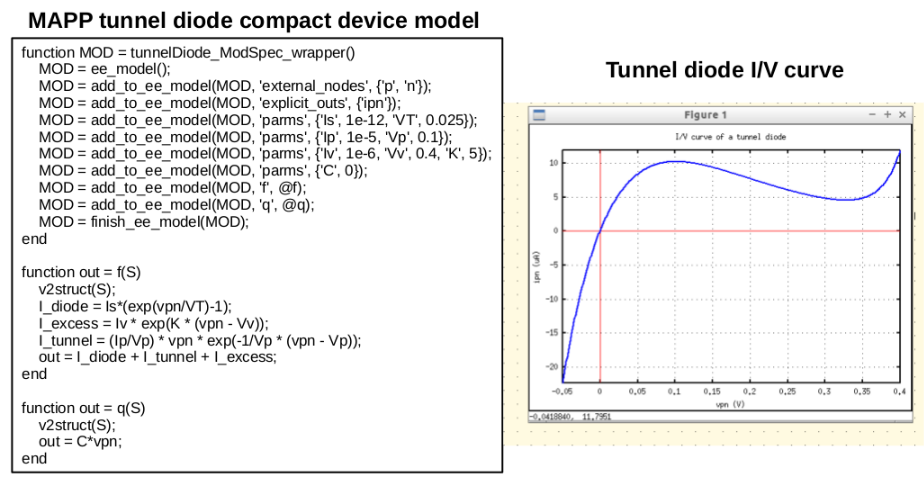
Figure 1.4. MAPP tunnel diode model and simulated diode current as a function of applied bias voltage.

The Qucs and MAPP modelling tools allow models represented by a set of mathematical equations based on the physical properties of a device to be tested and their correct operation confirmed prior to constructing a simulation model for inclusion in circuit schematics. Illustrated in Figure 1.5 is a third model for the tunnel diode plus a test circuit for simulating the device DC current versus voltage characteristics. This model will work with Qucs-0.0.18 and spice4qucs versions of the circuit simulator. It shows how a Qucs EDD model represents the physical model of the tunnel diode and how this model can be represented with it’s own symbol and tested by combining it with other components to form a DC characteristic test circuit. The Qucs EDD is not implemented in SPICE simulators. SPICE 3f5 and later simulators have instead other features like, for example, the B type sources.

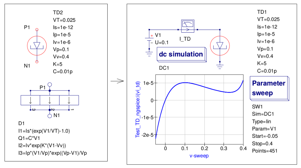
Figure 1.5. Qucs EDD behavioural model for the tunnel diode first introduced in Figure 1.3.

The Qucs EDD component has one feature which makes it particularly important for developing compact device simulation models, namely that its structure and modelling capabilities are similar to those available with the Verilog-A hardware description language. Hence, once an MAPP/Qucs EDD model is operating satisfactorily it can be transcribed into a Verilog-A compact model by inspection or by computer synthesis. Such a Verilog-A model and test circuit is shown in Figure 1.6.

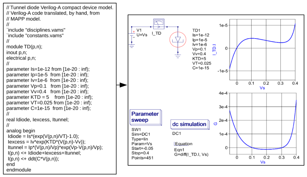
Figure 1.6. A Verilog-A compact tunnel diode model and test circuit.

One of the main aims of the spice4qucs initiative is both to improve the Qucs compact device modelling capabilities and to streamline the flow of information between each part of the modelling and simulation sequence. In all Qucs releases prior to the spice4qucs project a number of modelling tools were implemented in the distribution software but users had to translate manually each type of model format to other formats if they wished to use a model with a different simulator or modelling tool. One exception was the rudimentary translation tool called qucsconv for translating SPICE netlists to Qucs netlist format. It was for example not possible to simulate Qucs models encoded in the Qucs netlist format directly with a SPICE simulator or to generate a Verilog-A code model directly from a Qucs EDD model. This situation will change significantly as the spice4qucs project moves forward: in the medium to long term a number of synthesis-translation routines will be added to Qucs making the process of model translation transparent to the Qucs user. The first of these is the link between the Qucs netlist format and the Ngspice, Xyce and SPICE OPUS simulator netlist formats. Figure 1.5 shows a Qucs tunnel diode EDD model, a DC swept parameter test circuit and a set of Ngspice simulation results. Figure 1.7 lists an Ngspice netlist generated automatically by spice4qucs for the circuit shown in Figure 1.5. Notice that this netlist is not simply a list of SPICE component statements but includes an embedded Ngnutmeg script between the SPICE .control .... and .... .endc statements.

* Qucs 0.0.19  
* Qucs 0.0.19  TD.sch
.SUBCKT TD _net0 _net1 VT=0.025 Is=1e-12 Ip=1e-5 Iv=1e-6 Vp=0.1 Vv=0.4 K=5 C=0.01p 
BD1I0 _net0 _net1 I=Is*(exp((V(_net0)-V(_net1))/VT)-1.0)
GD1Q0 _net0 _net1 nD1Q0 _net1 1.0
LD1Q0 nD1Q0 _net1 1.0
BD1Q0 nD1Q0 _net1 I=-(C*(V(_net0)-V(_net1)))
BD1I1 _net0 _net1 I=Iv*exp(K*((V(_net0)-V(_net1))-Vv))
BD1I2 _net0 _net1 I=Ip*((V(_net0)-V(_net1))/Vp)*exp((Vp-(V(_net0)-V(_net1)))/Vp)
.ENDS
XTD2  _net0 0 TD VT=0.025 Is=1E-12 Ip=1E-5 Iv=1E-6 Vp=0.1 Vv=0.4 K=5 C=0.01P
VI_TD1 _net1 _net0 DC 0 AC 0
V1 _net1 0 DC 0.1
.control
set filetype=ascii
DC V1 -0.05 0.4 0.000997783
write _dc.txt VI_TD1#branch 
destroy all
exit
.endc
.END

Figure 1.7. A synthesized Ngspice netlist for the tunnel diode circuit shown in Figure 1.5.

Figure 1.8, and the associated model code, introduce a user defined XSPICE Code Model for the tunnel diode example. A recent extension to the spice4qucs compact device modelling capabilities adds a “turn-key” feature which allows user defined XSPICE Code Models to be added to Qucs and automatically compiled to C code by the package. More on this topic and all the others introduced earlier in this chapter can be found in later sections of this document.

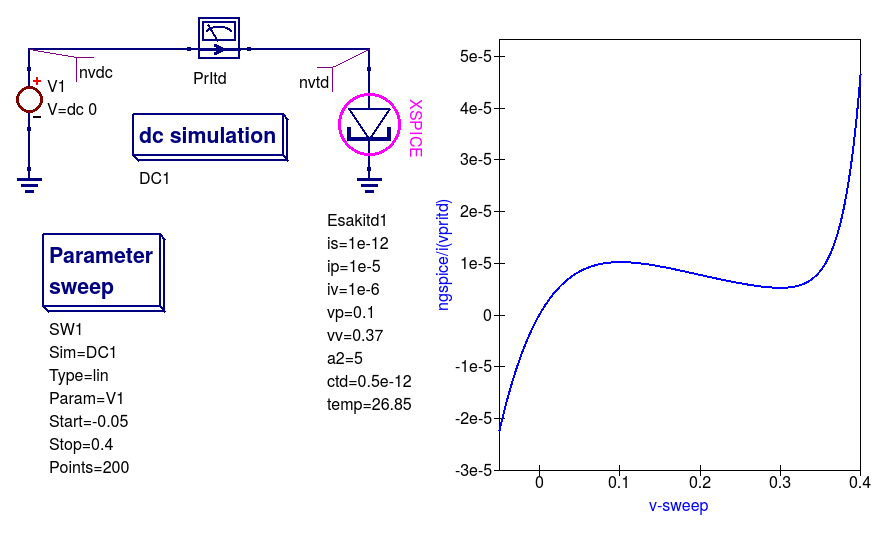
Figure 1.8. XSPICE Code Model tunnel diode model, test circuit and Ngspice simulation results.

/*
     etd cm model.                    

    2 April 2016    Mike Brinson

        
    This is free software; you can redistribute it and/or modify
    it under the terms of the GNU General Public License as published by
    the Free Software Foundation; either version 2, or (at your option)
    any later version.
*/


#include <math.h>                                                

void cm_etd(ARGS)
{
    Complex_t  ac_gain1;
    static double  PVP, PIP, PVV, PIV, PA2;
    static double PIS, T2, con1, con2, con3, VT;
    double ith, ix, it, dith, dix, ditu; 
    static double  vtd, itd, diff; 
    double P_K, P_Q; 
             
     if (INIT) {
        PVP    = PARAM(vp); 
        PIP    = PARAM(ip);
        PVV    = PARAM(vv);
        PIV    = PARAM(iv);
        PA2    = PARAM(a2);
        PIS    = PARAM(is);
 
/*      Constants                     */  
            
        P_K    = 1.3806503e-23 ;     /* Boltzmann's constant in J/K */
        P_Q    = 1.602176462e-19;    /* Charge of an electron in C   */
        T2     = PARAM(temp)+237.15;
        VT     = P_K*T2/P_Q;         /* Thermal voltage at Temp in volts */
        con1   = PIV*PA2;
        con2   = PIS/VT;
        con3   = PIP/PVP;



     }

   if (ANALYSIS != AC) { 
         vtd  = INPUT(ntd);
         ith  = PIS*(exp( vtd/VT) -1.0);
         ix   = PIV*exp(PA2*(vtd-PVV));
         it   = PIP*(vtd/PVP)*exp(1-vtd/PVP);
         itd  = ith+ix+it;
         dith = con2*exp(vtd/VT);
         dix  = con1*exp(PA2*(vtd-PVV));
         ditu = con3*(1-vtd/PVP)*exp(1-vtd/PVP);
         diff = dith+dix+ditu;
         
         OUTPUT(ntd) = itd;
         PARTIAL(ntd, ntd) = diff; 

   }

  else {
       ac_gain1.real = diff;
       ac_gain1.imag = 0.0;
       AC_GAIN(ntd, ntd) = ac_gain1;
      
     }
              
}

back to the top